This blogpost discusses a beautiful way for solving the following interesting problem.
Example 1. If are independent and identically distributed random variables taking values in the set of real numbers then show that
The above result follows from the positive semi-definiteness of Here we discuss an alternate solution, which is due to professor Fedor Petrov.
Solution with comments (thanks to professor Fedor Petrov). Notice that the problem doesn’t assume finiteness or even existence of the mean of Echoing on the standard practice of checking the case of infinite means first, we first get rid of the case when (and hence ) has an infinite expected value. We leave this as an exercise for the readers.
Exercise 2. Prove the claim in Example 1 in the case when
So it suffices to consider the case when has a finite expected value. Keeping aside this simplification for some time, let us look at the problem in a different way. The problem presents a claim about two iid random variables and This might suggest that it might be reasonable to rewrite the problem as a claim about the common law of Letting denote the common law of we can rewrite the claim in Example 1 as follows.
For any arbitrary probability distribution on the real numbers one has whenever and are independent random variables each having law
Echoing on the general problem solving strategy of finding a sufficient criteria, one may like to find a claim which implies (1). A naive start would be to guess that the random variable is non-negative with probability one. But this is not true.
Exercise 3. Show that there exists iid random variables such that
However we have
Indeed, for any real numbers one has The next natural step would be to take expectations on both sides of (2) and use the iid-ness of to get which is not quite the same as what we wanted but only slightly different from it.
Let us amplify the above argument to get a proof. The key role will be played by the following somewhat popular inequality.
Claim 4. For any natural number and any arbitrary reals one has
Applying the inequality (3) to the sample points for jointly independent random variables having law and take expectation on both sides we get that
thanks to Exercise 2 we see that sending gives us the desired claim.
So it suffices to prove Claim 4. A standard way is to induce on
Exercise 5. Show (3) when and notice that there is nothing to prove if Now, assuming the claim true for every $n \le m$ for some we aim to prove the claim for To this end, replace each by for a fixed and notice that the right hand side of (3) remains unchanged; optimize in by minimizing the left hand side of (3) and use the induction hypothesis to get the claim.
This completes the proof.
Remark 6. An interesting fact is that the inequality (1) holds even for iid vector-valued random variables and but the proof is slightly more difficult. It involves a trick of writing magnitudes for vectors in terms of inner products with random unit vectors. Here is a quick summary of this trick, by professor Terence Tao.
A retrospective analysis of the above solution, shows us that, in some sense, we removed probability from the picture (in the sense of finding a deterministic problem which implies the original claim made for random variables). This is an example of a more general strategy of de-probabilizing a problem. We shall discuss more about this matter in a later blogpost.
Also the fact that we are using Euclidean norm plays a crucial role in Example 1. For more details on it, see this post by professor Russ Lyons. This point will be discussed in more details in a later blogpost.
The long title of the post might already lend some idea on the main focus of this blogpost. We are going to prove the following.
Proposition 1 Let be a sequence of real (or complex) valued random variables such that there is some increasing, continuous function with (i.e., grows strictly faster than linearly) and for some absolute constant and for all Then if converges almost surely to as then also converges to as .
Before we prove Proposition 1, we would like to remark that, in general, it is not true that almost sure convergence implies convergence of mean.
Example 2 Let and let for any natural number we define the random variable by setting Then clearly, converges to for all but still for all while .
In the example above, the sequence is bounded in mean, and in fact for any bounded linear function we have but clearly, there is no function with a strict superlinear growth for which the sequence has absolutely bounded means (see Exercise 3).
Exercise 3 If are the random variables as defined in Example 2, then show that there is no function with for which one has
In this regard, Proposition 1 is quite elegant as it allows us to conclude convergence of means from a condition just slightly stronger than linear boundedness of means, and this actually follows because the boundedness of means in the superlinear setting actually implies the uniform integrability of which is, thanks to the bounded convergence theorem, stronger than what we need to conclude the claim. I had a much longer proof of this claim, which is essentially equivalent to the following more slick proof by professor Yuval Peres.
Proof of Proposition 1. Thanks to the bounded convergence theorem, it suffices to show that as
To begin, notice that there is some such that for all For each define Then notice that one has for all natural numbers and any
taking expectation on both sides of the above line of display and sending gives us the uniform integrability of since as and this proves the claim.
In the special case, when is the function one obtains the much useful Theorem 25 from this blogpost by professor Terence Tao. In fact, Proposition 1 above was motivated by the ensuing remark after Theorem 25 on professor Tao’s blogpost. One classic application of Theorem 25 from professor Tao’s blogpost (together with Kolmogorov’s 0-1 law) is demonstrated in the proof of the opening proposition here. In a later blogpost I shall discuss consequences of Proposition 1 which are of a similar flavour.
Recently I finished updating the document on standard techniques one often finds useful in combinatorics, which I wrote long back, and promised to update regularly in due course of time. It just happened that, unfortunately for a while I got distanced from combinatorics and paused working on the document. It is still not complete, at least I feel that I have more to discuss in this document so it will see another or a few more updates, hopefully very soon.
The most recent draft can be found below, in the attached file.
Here is a problem from St. Petersburg Math olympiad. Like most Russian problems, the calculations are minimal and a trick is used. This is a problem I wrote on in AoPS forum (see [2]), and it was labeled as combinatorics. But is it really combinatorics? In my opinion, it could be classified as number theory or inequalities, or even algebra, because it uses elements of those subjects. I recalled a funny classification I came across regarding what combinatorics means. Here it is.
In Olympiad mathematics the topics are defined in the following way.
Routine functional equations and inequalities that use at least once Cauchy-Schwarz, kind of AM-GM, Jensen, Karamata, etc., etc. arecalled algebra.
Synthetic two-dimensional Euclidean geometry is calledgeometry.
Fermat’s little theorem, Cauchy totient function and modular arithmetic are number theory.
As some of you would know, I am going to begin my term as a PhD graduate student in the department of mathematics at Indiana University at Bloomington. I am all very excited about this, especially because my interim advisor there is professor Russell Lyons and the kind of problems he works on is exactly what has picqued my interests recently and also it feels great to know professor Russ because apparently our wavelengths match quite well.
As most of you know, I often post notes from courses I take on my blog. I would be doing the same, and in fact I plan to scribe all the mathematics and related lectures I attend at Indiana University and post them on my IU blog.
Being said that, it doesn’t mean that I would discontinue posting updates of my mathematical findings on this blog. As always, I am pretty confident that I would still engage in a significant amount of self studying (anyways it will be more required and relevant now), and so updates of all those would be posted here.

 are independent and identically distributed random variables taking values in the set
  of real numbers then show that
![\displaystyle \mathbf{E} [ | X + Y | ] \ge \mathbf{E} [ | X - Y | ] ~~~~~~~ (1).](https://s0.wp.com/latex.php?latex=%5Cdisplaystyle+%5Cmathbf%7BE%7D+%5B+%7C+X+%2B+Y+%7C+%5D+%5Cge+%5Cmathbf%7BE%7D+%5B+%7C+X+-+Y+%7C+%5D+%7E%7E%7E%7E%7E%7E%7E+%281%29.&bg=ffffff&fg=000&s=0&c=20201002)


![\mathbf{E} [ |X|] (= \mathbf{E} [ |Y| ]) = + \infty.](https://s0.wp.com/latex.php?latex=%5Cmathbf%7BE%7D+%5B+%7CX%7C%5D+%28%3D+%5Cmathbf%7BE%7D+%5B+%7CY%7C+%5D%29+%3D+%2B+%5Cinfty.&bg=ffffff&fg=000&s=0&c=20201002)


![\mathbf{E} [ | X +Y | ] \ge \mathbf{E} [ |X- Y|]](https://s0.wp.com/latex.php?latex=%5Cmathbf%7BE%7D+%5B+%7C+X+%2BY+%7C+%5D+%5Cge+%5Cmathbf%7BE%7D+%5B+%7CX-+Y%7C%5D&bg=ffffff&fg=000&s=0&c=20201002) whenever
whenever  are independent random variables each having law


![\mathbf{E} [ |X| ] + \mathbf{E} [ |X+Y| ] \ge \mathbf{E} [ |X-Y| ]](https://s0.wp.com/latex.php?latex=%5Cmathbf%7BE%7D+%5B+%7CX%7C+%5D+%2B++%5Cmathbf%7BE%7D+%5B+%7CX%2BY%7C+%5D+%5Cge++%5Cmathbf%7BE%7D+%5B+%7CX-Y%7C+%5D&bg=ffffff&fg=000&s=0&c=20201002)
 and any arbitrary reals
  one has
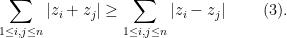


![\displaystyle \mathbf{E} [ |X + Y| ] + \frac{\mathbf{E} [ 2 |X| ]}{n-1} \ge \mathbf{E} [ |X-Y|] ~~~~~~~ (4);](https://s0.wp.com/latex.php?latex=%5Cdisplaystyle+%5Cmathbf%7BE%7D+%5B+%7CX+%2B+Y%7C+%5D+%2B+%5Cfrac%7B%5Cmathbf%7BE%7D+%5B+2+%7CX%7C+%5D%7D%7Bn-1%7D+%5Cge+%5Cmathbf%7BE%7D+%5B+%7CX-Y%7C%5D+%7E%7E%7E%7E%7E%7E%7E+%284%29%3B&bg=ffffff&fg=000&s=0&c=20201002)


and notice that there is nothing to prove if
Now, assuming the claim true for every $n \le m$ for some
we aim to prove the claim for
To this end, replace each
by
for a fixed
and notice that the right hand side of (3) remains unchanged; optimize in

but the proof is slightly more difficult. It involves a trick of writing magnitudes for vectors in terms of inner products with random unit vectors. Here is a quick summary of this trick, by professor Terence Tao.

 be a sequence of real (or complex) valued random variables such that there is some increasing, continuous function
  with
with  (i.e.,
  grows strictly faster than linearly) and
 ![\mathbf{E} [ | f( |X_n | ) | ] < M](https://s0.wp.com/latex.php?latex=%5Cmathbf%7BE%7D+%5B+%7C+f%28+%7CX_n+%7C+%29+%7C+%5D+%3C+M&bg=ffffff&fg=000&s=0&c=20201002) for some absolute constant
for some absolute constant  and for all
 converges almost surely to
  as
as ![\mathbf{E} [ X_n ]](https://s0.wp.com/latex.php?latex=%5Cmathbf%7BE%7D+%5B+X_n+%5D&bg=ffffff&fg=000&s=0&c=20201002) also converges to
also converges to  as
as ![\Omega = [0,1]](https://s0.wp.com/latex.php?latex=%5COmega+%3D+%5B0%2C1%5D&bg=ffffff&fg=000&s=0&c=20201002) and let for any natural number
and let for any natural number ![X_n ( \omega ) = n \mathbf{1}_{ \omega \in (0, 1/n] }.](https://s0.wp.com/latex.php?latex=X_n+%28+%5Comega+%29+%3D+n+%5Cmathbf%7B1%7D_%7B+%5Comega+%5Cin+%280%2C+1%2Fn%5D+%7D.&bg=ffffff&fg=000&s=0&c=20201002)
 converges to
  for all
 ![\omega \in [0,1]](https://s0.wp.com/latex.php?latex=%5Comega+%5Cin+%5B0%2C1%5D&bg=ffffff&fg=000&s=0&c=20201002) but still
but still ![\mathbf{E} [ X_n ] = 1](https://s0.wp.com/latex.php?latex=%5Cmathbf%7BE%7D+%5B+X_n+%5D+%3D+1&bg=ffffff&fg=000&s=0&c=20201002) for all
for all ![\mathbf{E} [ 0 ] = 0](https://s0.wp.com/latex.php?latex=%5Cmathbf%7BE%7D+%5B+0+%5D+%3D+0&bg=ffffff&fg=000&s=0&c=20201002) .
. is bounded in mean, and in fact for any bounded linear function
 ![\sup _n \mathbf{E} [ |f(X_n)| ] < \infty](https://s0.wp.com/latex.php?latex=%5Csup+_n+%5Cmathbf%7BE%7D+%5B+%7Cf%28X_n%29%7C+%5D+%3C+%5Cinfty&bg=ffffff&fg=000&s=0&c=20201002) but clearly, there is no function
but clearly, there is no function  has absolutely bounded means (see
  for which one has
 ![\sup_n \mathbf{E} [ f(X_n) ] < \infty.](https://s0.wp.com/latex.php?latex=%5Csup_n+%5Cmathbf%7BE%7D+%5B+f%28X_n%29+%5D+%3C+%5Cinfty.&bg=ffffff&fg=000&s=0&c=20201002)
 which is, thanks to the
 ![\sup_n \mathbf{E} [ |X_n| \mathbf{1}_{|X_n| > m } ] \to 0](https://s0.wp.com/latex.php?latex=%5Csup_n+%5Cmathbf%7BE%7D+%5B+%7CX_n%7C+%5Cmathbf%7B1%7D_%7B%7CX_n%7C+%3E+m+%7D+%5D+%5Cto+0&bg=ffffff&fg=000&s=0&c=20201002) as
as 
 such that
  for all
  For each
  define
 and any

 gives us the uniform integrability of
  since
since  as
as  and this proves the claim.
  one obtains the much useful Theorem 25 from